Workflow

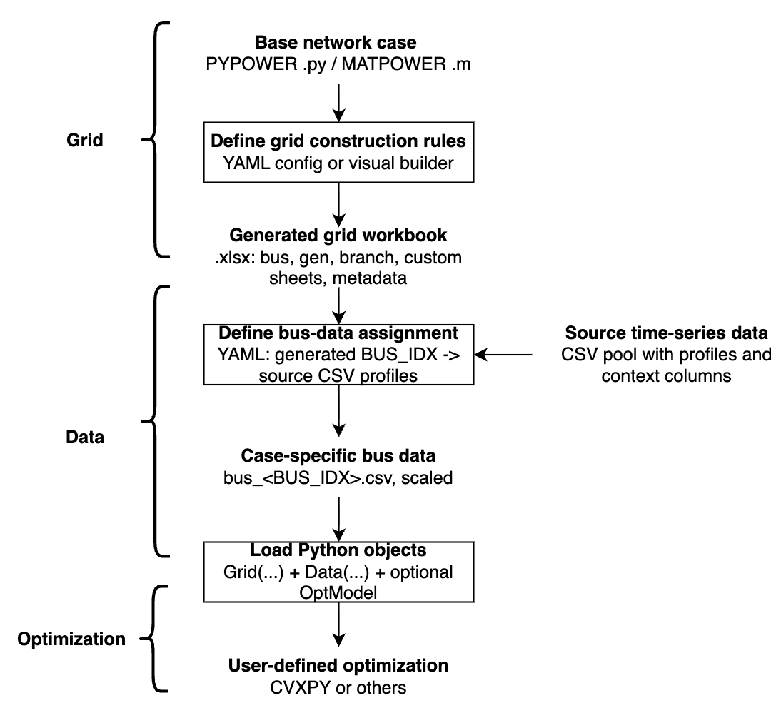
GridForge turns a base power-system case into optimization-ready Python data in four stages:

1. Static grid construction
   User-defined YAML rules + MATPOWER/PYPOWER base case -> Full Excel workbook

2. Time-series assignment
   source data pool + assignment config YAML -> case-specific bus_<BUS_IDX>.csv files

3. Python access
   Excel workbook -> Grid(...) class instance
   case-specific CSVs -> Data(...) class instance

4. Optimization
   Grid + Data -> user-defined optimization model in CVXPY or another optimization tool

GridForge also comes with a ready-to-use dataset from TX-123BT system which is a synthetic Texas power system with time-series weather-dependent spatiotemporal profiles.

Note: TX-123BT is optional. It is one example source for producing a pool of per-bus CSV files, not a signal for GridForge itself.

Stage 1: Build The Grid Workbook

GridForge starts from a PYPOWER/MATPOWER-style case and applies YAML rules. The YAML file describes static changes: which columns to overwrite, which custom asset sheets to create, where those assets sit in the network, and how totals should be rescaled.

The user should specify the name of a pypower case or a local PYPOWER/MATPOWER-sytle case file in .py or .m format. The user can then modify the grid configuration by adding or modifying grid assets with YAML files.

The YAML can be written manually or created with the Visual Config App.

Once the yaml file is ready, the user can construct the grid configuration by running the following code:

from gridforge.construct import construct_grid_config

construct_grid_config(
    "examples/14bus_uc/14bus_config.yaml",  # user-defined YAML rules
    "examples/14bus_uc/14bus_config.xlsx",  # output Excel workbook
    random_seed=404,
)

The generated Excel workbook contains core sheets: bus, gen, and branch.

and any custom asset sheets attached to buses, such as:load, solar, wind, storage, etc.

Generator cost data from PYPOWER/MATPOWER gencost is merged into gen as COST_* columns, for example COST_STARTUP, COST_FIRST, and COST_ZERO.

For the full YAML schema, see configuration.md.

Stage 2: Assign Bus Data

The grid config decides which assets exist and where they sit. Time-series data is attached later through a separate bus-level assignment file, so static assets do not automatically require CSV data.

Only workbook sheets referenced by signals.<name>.workbook_sheet are treated as data-backed. For each signal, GridForge reads that sheet's BUS_IDX values from the Excel workbook to know which generated buses require data.

from gridforge.data import (
    load_bus_data_assignment,
    materialize_bus_data_assignment,
    suggest_bus_data_assignment,
)

assignment_template = load_bus_data_assignment("examples/14bus_uc/14bus_data_assignment.yaml")
assignment = suggest_bus_data_assignment(
    grid_xlsx_path="examples/14bus_uc/14bus_config.xlsx",
    source_data_dir="data/bus_data",
    signals=assignment_template["signals"],
    output_data_dir="examples/14bus_uc/14bus_data",
    random_seed=404,
)

materialize_bus_data_assignment(
    grid_xlsx_path="examples/14bus_uc/14bus_config.xlsx",  # input Excel workbook from Stage 1
    assignment=assignment,  # generated bus-to-source mapping
    output_data_dir="examples/14bus_uc/14bus_data",  # output directory for case-specific bus_<BUS_IDX>.csv files
)

This reads source data files and writes case-specific files such as:

examples/14bus_uc/14bus_data/bus_2.csv
examples/14bus_uc/14bus_data/bus_3.csv

For assignment schema, scaling rules, and suggested mappings, see bus-data-assignment.md.

Stage 3: Load Grid And Data

from gridforge.opt import Grid, Data

grid = Grid(
    "examples/14bus_uc/14bus_config.xlsx",  # input Excel workbook from Stage 1
    verbose=0,
)

data = Data(
    grid_xlsx_path="examples/14bus_uc/14bus_config.xlsx",  # input Excel workbook from Stage 1
    data_dir="examples/14bus_uc/14bus_data",  # input directory for case-specific bus_<BUS_IDX>.csv files
    sheet_names=["load", "solar", "wind"],
)

Grid(...) exposes the static workbook as arrays, DataFrames, and incidence matrices:

• grid.sheets[...]: raw Excel sheets as pandas DataFrames
• grid.core.*: schema-defined core sheets
• grid.custom[...]: generic custom sheets attached to buses
• aliases such as grid.gen, grid.branch, grid.load, and grid.solar

Data(...) loads time-series matrices aligned to the workbook row order. This alignment is what lets grid.load.Cbus @ load[t] map a time-series vector to bus injections correctly.

For detailed access patterns, see grid-data-access.md.

Stage 4: Build An Optimization Model

GridForge does not prescribe a fixed optimization model. You can use Grid, Data, and OptModel to assemble your own formulation in CVXPY or another optimization tool.

import cvxpy as cp
from gridforge.opt import OptModel

T = 24
m = OptModel(grid)

m.add_variable("pg", (T, grid.gen.n))
m.add_parameter("load", (T, grid.load.n))

pg = m.vars["pg"]
load = m.params["load"]

for t in range(T):
    injection = grid.gen.Cbus @ pg[t] - grid.load.Cbus @ load[t]
    m.add_constraint([
        cp.sum(injection) == 0,
        grid.branch.ptdf @ injection <= grid.branch.pmax / grid.baseMVA,
        grid.branch.ptdf @ injection >= -grid.branch.pmax / grid.baseMVA,
    ])

prob = m.compile(load=data.get_series("load")[:T, :] / grid.baseMVA)

The full unit-commitment example is in 14bus_example.py.

Visual Config App

The Streamlit app is a visual YAML builder for Stage 1. It edits the same YAML format used by construct_grid_config(...).

gridforge-app

From a local checkout:

streamlit run gridforge/config_app.py

For installation notes and the boundary between the visual app and bus-data assignment, see visual-app.md.

Optional TX-123BT Source Data

GridForge includes an optional TX-123BT workflow that prepares a public source CSV pool under data/bus_data/.

bash scripts/generate_tx123bt_bus_data.sh

This is not required for GridForge. It is one example data source that can feed the generic bus-data assignment step.

For details, see tx123bt.md.